The Magic of Variational Inference
Introduction
Hi guys, welcome to my blogpost again :) Today, I want to discuss about the magical and how wonderful Variational Inference (VI) is. This approach is widely used in many applications, such as text-to-image generation, motion planning, Reinforcement Learning (RL), etc.
The reason for this is that in many cases the distribution of generated output that we want is very complex, e.g., images, text, video, etc. This is where VI can help us through latent variables. I believe that once we can master this concept well, then we can understand many recent AI techniques more easily and intuitively.
I often found the explanation on the internet about this topic is not clear enough in explaining the reasons why this concept needs to exist somehow, why we need to calculate many fancy math terms, etc. Therefore, in this post I also want to focus more on the reasoning part so that all of us can understand the essence of this method beyond the derivations and usefulness of VI.
This post is based on my understanding of the topic, so if you find any mistake please let me know :)

Latent Variable Models
You may ask what Variational Inference (VI) really is? How it can be oftenly used in many recent AI methods? To answer those questions, let me start with latent variable models.
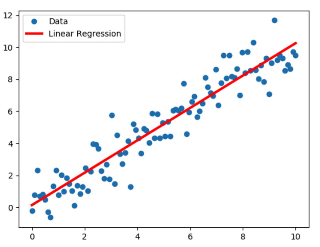
Let’s say we want to build a regression model that can fit a simple data distribution like this,

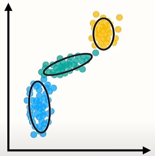
What we basically try to do from the image above is to model \(p(\mathbf{y} \mid \mathbf{x})\) where \(y\) is our data given \(x\). It seems very simple right? But now let’s imagine we have quite complex data dsitribution like below,

You might be confused initially on how we can build a model that fits that distribution. But don’t worry, I was also used to be like that too :) In reality, the distribution that we face might be much more complex than that.
Fortunately, we can approximate that distribution through multiplication of two simple distributions. How we can do that? This is where the concept of latent variable models comes into play.
The data distribution itself \(p(\mathbf{x})\) can be expressed mathematically as,
\[p(\mathbf{x})=\sum_z p(\mathbf{x} \mid \mathbf{z}) p(\mathbf{z})\]where \(\mathbf{z}\) is the latent variable. Maybe you ask, what is that thing? Basically it is the hidden value that is not the variable \(y\) nor \(x\), but needs to be considered where we want to calculate the probability of the observed data \(\mathbf{x}\) in a more complex distribution. These latent variables represent underlying factors or characteristics that might not be directly observable but significantly influence the observed data.
For example, the latent variables for figure 3 is the categorical value that maps each data point into cluster blue, green, or yellow.
You may still wonder, how latent variable models is used in this case? First, we need to know that the prior or latent variable distribution \(p(\mathbf{z})\) is assumed to be a simple distribution, typically chosen as a standard gaussian distribution \(\mathcal{N}\left(0, \boldsymbol\Sigma^{2}\right)\), with variance \(\boldsymbol\Sigma^{2}\).
So how about the distribution \(p(\mathbf{x} \mid \mathbf{z})\)? This is also assumed to be a normal distribution, but the parameters mean \(\boldsymbol\mu_{nn}\) and the variance \(\boldsymbol\Sigma_{nn}^{2}\) are generated by our neural networks. This means that even though the process of defining that distribution can be quite complex, but it is still considered to be a simple distribution since we can parameterize it.
Thus, by doing like that we basically can approximate our data distribution \(p(\mathbf{x})\) as the multiplication of two simple distributions \(p(\mathbf{x})= \sum_z p(\mathbf{x} \mid \mathbf{z}) p(\mathbf{z})\). This is why we use latent variable models.
But, there is a problem when we use this approach directly. Remember that earlier we assumed that the prior distribution \(p(\mathbf{z})\) is just a standard gaussian distribution which also means that it is a unimodal distribution.
Can you imagine if we leverage that simple distribution directly without any training or learning process to approximate a very complex distribution which is oftenly has many modes? What will happen is that the approximation result will be not good since we do not incorporate any knowledge about our data into the pre-defined prior distribution. This is the where VI plays an important role :)
Posterior Distribution
From the previous explanation, you may be curious on how to update our prior belief represented by \(p(\mathbf{z})\). Actually, bayes theorem provides a way to do that. Specifically, the answer lies on what we call as posterior distribution \(p(\mathbf{z} \mid \mathbf{x})\). But in many cases, we cannot compute that expression or even if we can, then we need a lot of resources.
For understanding why is that, let me briefly recap about the use of bayes theorem in this case.
Our posterior can mathematically be expressed as,
\[p(\mathbf{z} \mid \mathbf{x}) = \frac{p(\mathbf{x} \mid \mathbf{z}) \, p(\mathbf{z})}{p(\mathbf{x})}\]where \(p(\mathbf{x})\) is the marginal likelihood or evidence of our data distribution.
There is also a joint distribution \(p(\mathbf{z}, \mathbf{x})\) that represents the probability of both the latent variables \(\mathbf{z}\) and the observed data \(\mathbf{x}\) occurring together. It can be factored into the product of the likelihood and the prior:
\[p(\mathbf{z}, \mathbf{x}) = p(\mathbf{x} \mid \mathbf{z}) \, p(\mathbf{z})\]To calculate the marginal likelihood \(p(\mathbf{x})\), we can view it from bayesian perspective as the probability of observing the data \(\mathbf{x}\) marginalized over all possible values of the latent variables \(\mathbf{z}\). It is obtained by integrating (or summing, in the case of discrete variables) the joint distribution over \(\mathbf{z}\):
\[p(\mathbf{x}) = \int p(\mathbf{z}, \mathbf{x}) \, \mathrm{d}\mathbf{z} = \int p(\mathbf{x} \mid \mathbf{z}) \, p(\mathbf{z}) \, \mathrm{d}\mathbf{z}\]This integral accounts for all possible configurations of the latent variables that could have generated the observed data.
So why \(p(\mathbf{z} \mid \mathbf{x})\) is very difficult to calculate? The reason is that if we want to calculate it, then it means that we also need to calculate \(p(\mathbf{x})\) since it is located in the denominator of the posterior math equation. This also means that the complexity will arise rapidly as the dimensionality of \(\mathbf{z}\) grows.
This is because the integral used for calculating \(p(\mathbf{x})\) sums over all possible values of \(\mathbf{z}\), and each evaluation of the joint distribution within the integral can also be computationally expensive, leading to an intractable integral.
For example, let’s imagine we have a mixture model with \(K = 2\) clusters as our latent variable and \(n = 3\) data points which represents our observed data \(\mathbf{x}\). Thus, we will have 8 combinations as follows: (1,1,1), (1,1,2), (1,2,1), (1,2,2), (2,1,1), (2,1,2), (2,2,1), (2,2,2). Here, each tuple represents the cluster assignments for the three data points.
For each of the 8 combinations of cluster assignments, we have to evaluate the likelihood of the entire data set given these assignments and the cluster means. The integral for every combination will be a two-dimensional integral over the two means (\(\mu_1\) and \(\mu_2\)). Then, the integral for marginal distribution can be written as,
\[p(\mathbf{x}) = \int \int \prod_{i=1}^{3} p(x_i \mid \mu_{c_i}) \, p(\mu_1) \, p(\mu_2) \, d\mu_1 \, d\mu_2\]Here, \(p(x_i \mid \mu_{c_i})\) represents the likelihood of data point \(x_i\) given the mean of its assigned cluster \(\mu_{c_i}\), where \(c_i\) is the cluster assignment for data point \(i\).
Notice that the number of integral follows the total dimensions that our latent variable \(\mathbf{z}\) has. In reality, we can have up to thousands of latent dimensions which means that we need to calculate thousands-dimensional integral!!
Even for our very simple example, the cost can be computationally intensive, particularly when the likelihood and prior distributions do not have closed-form solutions!!
Note* : closed-form solutions refers to the exact results from using standard math operations.
Approximate Posterior Distribution
Now you understand why calculating the exact posterior distribution is often very difficult. Many researchers try to solve this problem by approximating that distribution in various ways. In this post, I just want to focus on the estimation method related to the VI concept. Let’s go into more detail yeeyy :)
Remember that the root cause is not the posterior itself, but its requirement to calculate marginal distribution \(p(\mathbf{x})\) to derive \(p(\mathbf{z} \mid \mathbf{x})\) which involves integrations. Thus, the key idea here is to approximate the posterior by replacing the annoying integral operations with the optimization process of expected value \(E_{z \sim q_i(\mathbf{z})}\) with respect to approximate posterior \(q_i(\mathbf{z})\).
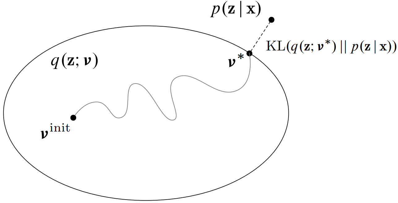
Specifically, the optimization is used to find the best approximation \(q_i(\mathbf{z} ; \boldsymbol{v*})\) where \(\boldsymbol{v*}\) are the variational parameters from a chosen family of distributions that minimizes the difference (specifically, the Kullback-Leibler divergence) from the true posterior \(p(\mathbf{z} \mid \mathbf{x})\).

So how we can do that approximation? First recall that the marginal distribution can be expressed as,
\[p(\mathbf{x}) = \int p(\mathbf{x} \mid \mathbf{z}) \, p(\mathbf{z}) \, \mathrm{d}\mathbf{z}\]That above equation can also be written as,
\[p(\mathbf{x}) = \int p(\mathbf{x} \mid \mathbf{z}) \, p(\mathbf{z}) \, \mathrm{d}\mathbf{z} = \int p(\mathbf{x} \mid \mathbf{z}) \, p(\mathbf{z}) \, \frac{q_i(\mathbf{z})}{q_i(\mathbf{z})} \, \mathrm{d}\mathbf{z}\]The introduction of \(\frac{q_i(\mathbf{z})}{q_i(\mathbf{z})}\) is a mathematical trick that allows us to rewrite the marginal likelihood in terms of the variational distribution \(q_i(\mathbf{z})\). By doing this, we can utilize the expected value with respect to \(q_i(\mathbf{z})\) to approximate the integral.
The modified expression for the marginal likelihood becomes,
\[p(\mathbf{x}) = \int q_i(\mathbf{z}) \, \frac{p(\mathbf{x} \mid \mathbf{z}) \, p(\mathbf{z})}{q_i(\mathbf{z})} \, \mathrm{d}\mathbf{z}\]The above expression can be interpreted as the expected value of the ratio \(\frac{p(\mathbf{x} \mid \mathbf{z}) \, p(\mathbf{z})}{q_i(\mathbf{z})}\) under the variational distribution \(q_i(\mathbf{z})\). Therefore, we can write like this,
\[p(\mathbf{x}) = E_{\mathbf{z} \sim q_i(\mathbf{z})}\left[\frac{p(\mathbf{x} \mid \mathbf{z}) \, p(\mathbf{z})}{q_i(\mathbf{z})}\right]\]By using this formulation, we can avoid the direct computation of the integral for the marginal likelihood, which is typically intractable. Instead, we use optimization problem for finding the optimal \(q_i(\mathbf{z})\) that minimizes the difference from the true posterior involving expected value calculation.
This approach is the essence of variational inference, transforming a challenging integration problem into a more manageable optimization problem. Specifically, we want to move difficult optimization
\[q_i^*(\mathbf{z})=\underset{q_i(\mathbf{z}) \in Q}{\operatorname{argmin}}(D_{\mathrm{KL}}(q_i(\mathbf{z} ; \boldsymbol{v}) \| p(\mathbf{z} \mid \mathbf{x})))\]since we do not have true posterior \(p(\mathbf{z} \mid \mathbf{x})\) into easier one by replacing KL divergence with variational lower bound \(\mathcal{L}_i\left(p, q_i^*\right)\) (Don’t worry, we will discuss this notation in more detail in the next section) like below,
\[q_i^*(\mathbf{z})=\underset{q_i(\mathbf{z}) \in Q}{\operatorname{argmax}}(\mathcal{L}_i\left(p, q_i^*\right))\]Evidence Lower Bound Objective (ELBO)
It turns out that if we approximate the true posterior by doing what we discussed before, then we can construct a lower bound for the marginal distribution \(p(x_i)\) of each \(x_i\) point. This can be a very powerful idea because by having that lower bound we can also maximize the loglikelihood of \(p(x_i)\).
Note that generally increasing the lower bound does not necessarily mean also increase the loglikelihood of \(p(x_i)\), but if some conditions are satisfied, then it does (we will discuss more about this later).
Recall that by looking at the previous equation, we can also derive the mathematical equation for each data point \(x_i\) of the distribution \(p(x_i)\) as,
\[p(x_i) = E_{\mathbf{z} \sim q_i(z)}\left[\frac{p(x_i \mid z) \, p(z)}{q_i(z)}\right]\]If we apply log operation for both sides of the equation, we can get the expression like below,
\[\log p\left(x_i\right) = \log E_{z \sim q_i(z)}\left[\frac{p\left(x_i \mid z\right) p(z)}{q_i(z)}\right]\]Then, we can implement jensen’s inequality \(\log E[y] \geq E[\log y]\) into our case, then we can get,
\[\log p\left(x_i\right) \geq E_{z \sim q_i(z)}\left[\log \frac{p\left(x_i \mid z\right) p(z)}{q_i(z)}\right]\]By leveraging log property, the above equation can also be expressed as,
\[\log p\left(x_i\right) \geq E_{z \sim q_i(z)}\left[\log p\left(x_i \mid z\right)+\log p(z)\right] - E_{z \sim q_i(z)}\left[\log q_i(z) \right]\]where \(- E_{z \sim q_i(z)}\left[\log q_i(z) \right]\) is the entropy \(\mathcal{H}\left(q_i\right)\). The above inequality is also called as variational lower bound \(\mathcal{L}_i\left(p, q_i\right)\).
So how we can make that lower bound to be tighter? The answer lies on how we can find a good approximation for \(q_i(z)\). So how we can do that? Yes you are right, the answer is by using KL divergence!
The mathematical equation for implementing KL divergence between approximate and the true posterior can be written like this,
\[D_{\mathrm{KL}}\left(q_i\left(x_i\right) \| p\left(z \mid x_i\right)\right) = E_{z \sim q_i(z)}\left[\log \frac{q_i(z)}{p\left(z \mid x_i\right)}\right]\]For those who are not familiar with KL divergence before, so basically the equation above measures how one probability distribution diverges from a second, expected probability distribution.
Recall that the bayes theorem tells us,
\[p(z \mid x_i) = \frac{p(x_i \mid z) p(z)}{p(x_i)}\]Therefore, we can use that to rewrite the term inside our KL divergence as:
\[\frac{q_i(z)}{p\left(z \mid x_i\right)} = \frac{q_i(z)}{\frac{p(x_i \mid z) p(z)}{p(x_i)}} = \frac{q_i(z) p(x_i)}{p(x_i, z)}\]where \(p(x_i \mid z) p(z) = p(x_i, z)\) is derived from the definition of joint probability. By inserting above expression into inside our KL divergence, we can get,
\[D_{\mathrm{KL}}\left(q_i\left(x_i\right) \| p\left(z \mid x_i\right)\right) = E_{z \sim q_i(z)}\left[\log \frac{q_i(z) p\left(x_i\right)}{p\left(x_i, z\right)}\right]\]After that, by using the log property we can also write above equation as,
\[\begin{aligned} D_{\mathrm{KL}}\left(q_i\left(x_i\right) \| p\left(z \mid x_i\right)\right) = & -E_{z \sim q_i(z)}\left[\log p\left(x_i \mid z\right) + \log p(z)\right] \\ & + E_{z \sim q_i(z)}\left[\log q_i(z)\right] + E_{z \sim q_i(z)}\left[\log p\left(x_i\right)\right] \end{aligned}\]Since \(- E_{z \sim q_i(z)}\left[\log q_i(z) \right]\) is the entropy \(\mathcal{H}\left(q_i\right)\), we can also write,
\[\begin{aligned} D_{\mathrm{KL}}\left(q_i\left(x_i\right) \| p\left(z \mid x_i\right)\right) = & -E_{z \sim q_i(z)}\left[\log p\left(x_i \mid z\right) + \log p(z)\right] \\ & - \mathcal{H}\left(q_i\right) + \log p\left(x_i\right) \end{aligned}\]Then, we can also express above equation as,
\[D_{\mathrm{KL}}\left(q_i\left(x_i\right) \| p\left(z \mid x_i\right)\right) = -\mathcal{L}_i\left(p, q_i\right)+\log p\left(x_i\right)\]Rearranging above equation give us,
\[\log p\left(x_i\right) = D_{\mathrm{KL}}\left(q_i(z) \| p\left(z \mid x_i\right)\right)+\mathcal{L}_i\left(p, q_i\right)\]As you can see, from the equation above we can say that if we successfully minimize the KL divergence part into 0 (which means our approximate posterior is exactly same with the true one), then the loglikelihood of our marginal or data distribution is also exactly same with the variational lower bound \(\mathcal{L}_i\left(p, q_i\right)\).
Thus, we already have a way to make that lower bound more tight by minimizing the KL divergence part.
But, how we can minimize the KL divergence in order to make the lower bound to be more tighter? Notice that in the last equation for \(\log p\left(x_i\right)\) that we have derived before, \(\log p(x_i)\) is a constant with respect to (w.r.t.) the variational distribution \(q_i(z)\).
This means that if we maximize variational lower bound (we can also call it as ELBO at this step) with respect to \(q_i(z)\), then it also means we minimize \(D_{\mathrm{KL}}\left(q_i(z) \| p(z \mid x_i)\right)\) since \(\log p(x_i)\) is constant w.r.t. \(q_i(z)\).
Thus, we can say that we can make the lower bound more tight by maximizing ELBO with respect to \(q_i(z)\) since it minimizes KL divergence. Similarly, we can also maximizes our likelihood / model by maximizing the same ELBO w.r.t. \(p\).
Conclusion
After long discussion, you may still wonder what Variational Inference (VI) essentially tells us about? At its core, VI is a powerful method for making the intractable tractable. By introducing a variational distribution \(q_i(\mathbf{z})\) and optimizing it, VI transforms the challenging problem of computing the true posterior \(p(\mathbf{z} \mid \mathbf{x})\) into an optimization problem that is much more manageable computationally.
This transformation rely on the replacement of the computationally intensive KL divergence with the variational lower bound \(\mathcal{L}_i\left(p, q_i^*\right)\), or ELBO. The key idea here is that instead of directly handle the high-dimensional integrals to define the true posterior, we work with a surrogate optimization problem that is much easier to solve but still retains the essential characteristics of the original problem.
In essence, VI is about approximation and efficiency. By approximating the intractable posterior distribution with a more tractable form and maximizing the ELBO, we can indirectly estimate the true posterior.