Autonomous Driving Paper Review 1, HLS for Future Trajectory!
Introduction
Disclaimer : This review is based on my understanding of the reference paper [1]. While I have made much effort to ensure the accuracy of this article, there may things that I have not fully captured. If you notice any misinterpretation or error, please feel free to point them out in the comments section.
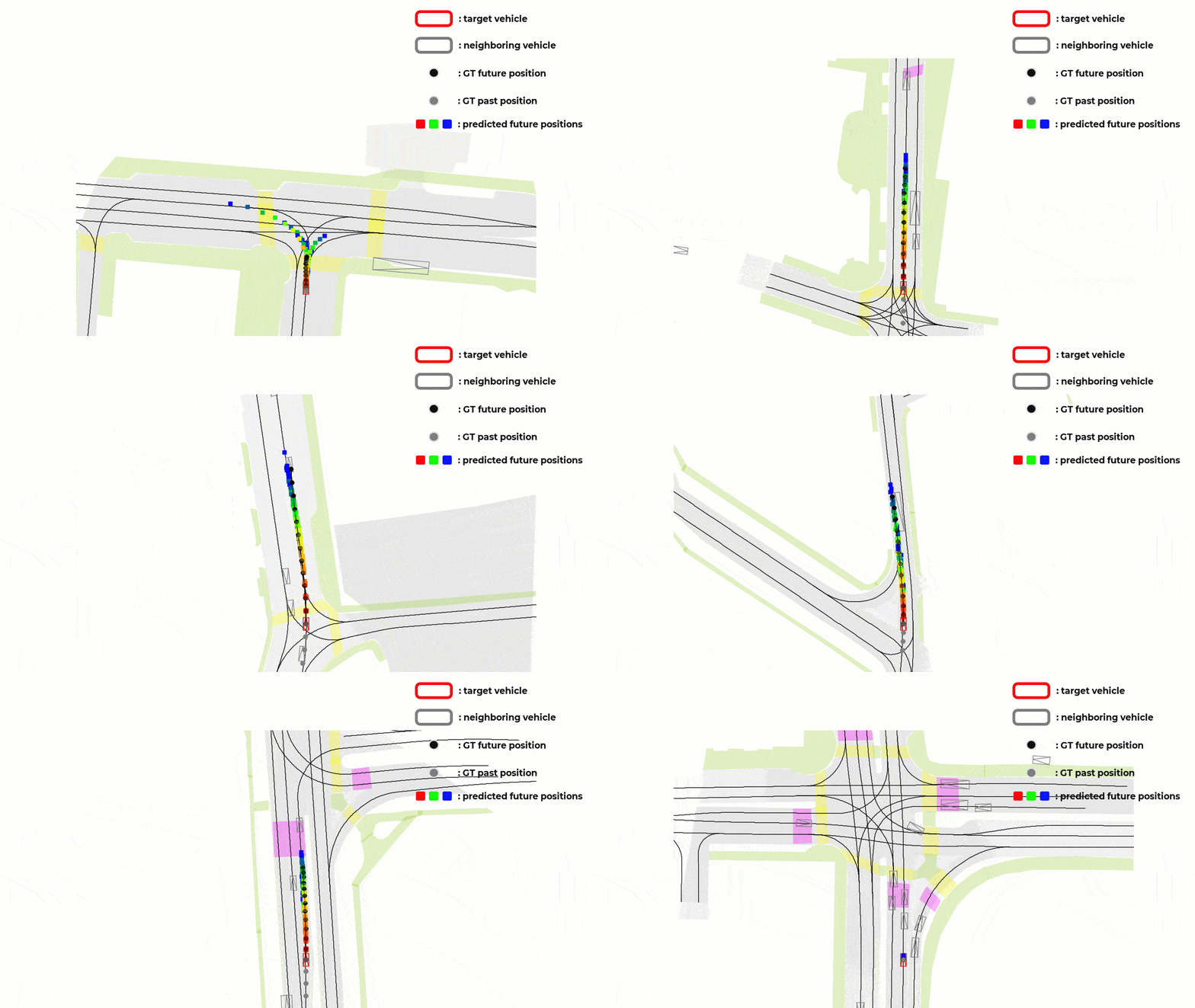
I’m very excited to present a review of the paper titled “Hierarchical Latent Structure for Multi-Modal Vehicle Trajectory Forecasting” [1] authored by Dooseop Choi and KyoungWook Min. This paper is a very good work proved by its acceptance at the European Conference on Computer Vision (ECCV) 2022.
For you who are not familiar with academia world in the AI field yet, ECCV is one of the most prestigious conferences in the domain. I truly believe this research paper is crucial for the autonomous driving topic, particularly in trajectory forecasting.
Notations and Definitions
| Notation | Definition |
|---|---|
| \(N\) | Number of vehicles in the traffic scene |
| \(T\) | Total number of timesteps for which trajectories are forecasted |
| \(H\) | Number of previous timesteps considered for positional history |
| \(V_{i}\) | The \(i^{th}\) vehicle in the traffic scene |
| \(\mathbf{Y}_{i}\) | Future positions of \(V_{i}\) for the next \(T\) timesteps |
| \(\mathbf{X}_{i}\) | Positional history of \(V_{i}\) for the previous \(H\) timesteps at time \(t\) |
| \(\mathcal{C}_{i}\) | Additional scene information available to \(V_{i}\) |
| \(\mathbf{L}^{(1: M)}\) | Lane candidates available for \(V_{i}\) at time \(t\) |
| \(\mathbf{z}_{l}\) | Low-level latent variable used to model the modes |
| \(\mathbf{z}_{h}\) | High-level latent variable used to model the weights for the modes |
| \(p_{\theta}\) | Decoder network |
| \(p_{\gamma}\) | Prior network |
| \(\mathcal{L}_{E L B O}\) | Modified ELBO objective |
| \(q_{\phi}\) | Approximated posterior network |
| \(f_{\varphi}\) | Proposed mode selection network |
VLI | Vehicle-Lane Interaction |
V2I | Vehicle-to-Vehicle Interaction |
The Main Problem : “Mode Blur”
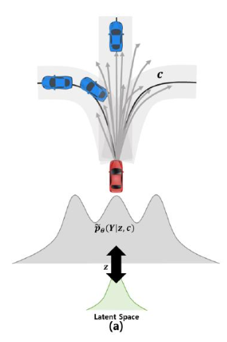
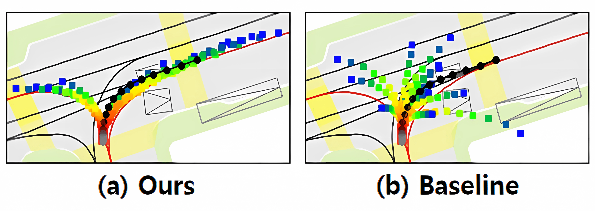
The paper aims to overcome a specific limitation in vehicle trajectory forecasting models that leverage Variational Autoencoders (VAEs) concept called as the “mode blur” problem. For clearer illustration, please take a look at the figure below (this corresponds to the figure 1 in the reference paper [1]) :
What is “Mode Blur” Problem?
As you can see from the figure above, the red vehicle is attempting to forecast its future trajectory represented by the branching gray paths. The challenge faced here lies in the generated forecast trajectories’ that are sometimes between defined lane paths.
This phenomenon is what the author mean by the “mode blur” problem. Specifically, the VAE-based model is not committing to a specific path, but rather giving a “blurred” average of possible outcomes.
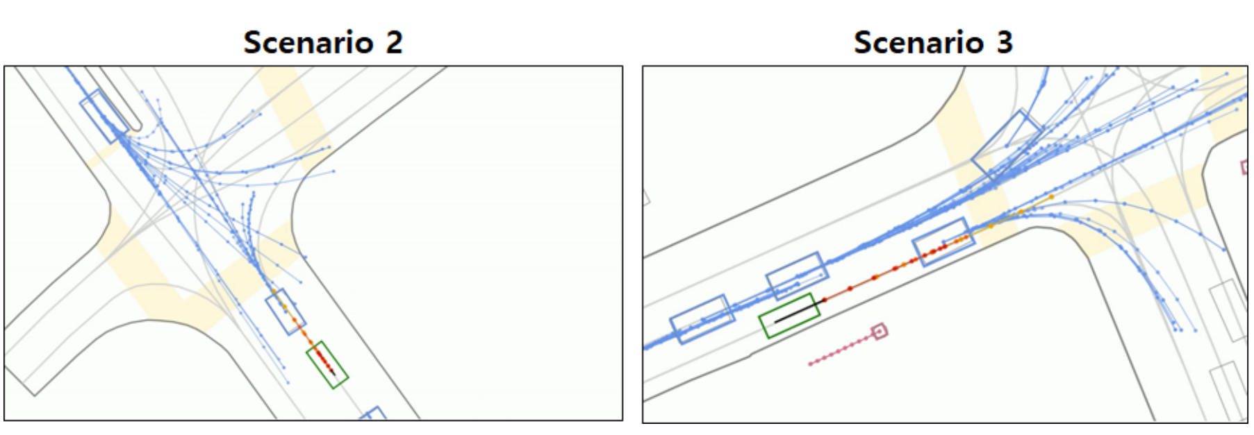
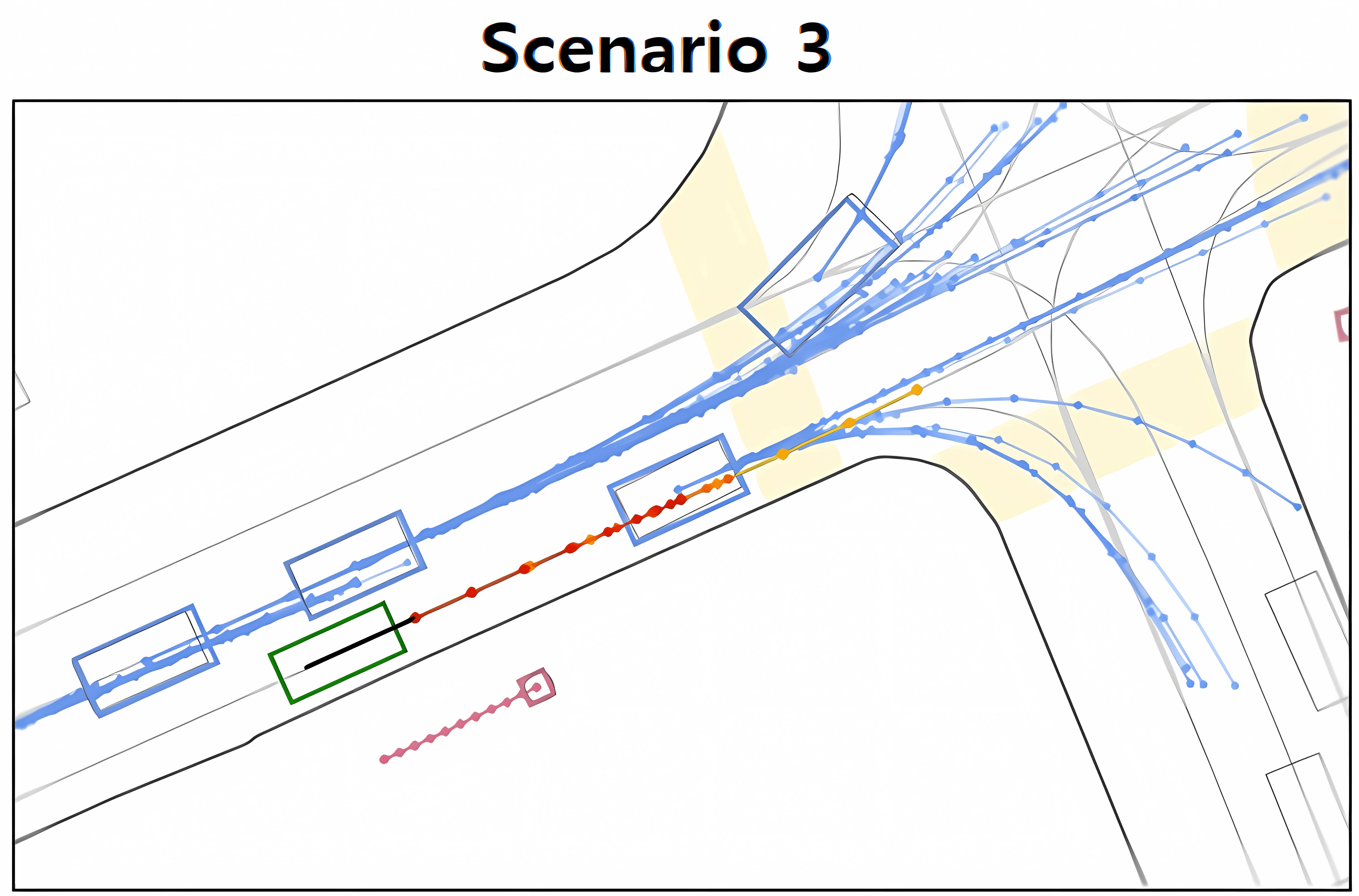
If you still wonder why the “mode blur” problem can be very important, consider the above figure example taken from the previous SOTA model as observed by D. Choi & K. Min [1]. Before analyzing that figure in more detail, assume that the green bounding box represents the Autonomous Vehicle (AV), the light blue bounding boxes represent surrounding vehicles, and the trajectories (path predictions) of the surrounding vehicles are shown using the solid lines with light blue dots.
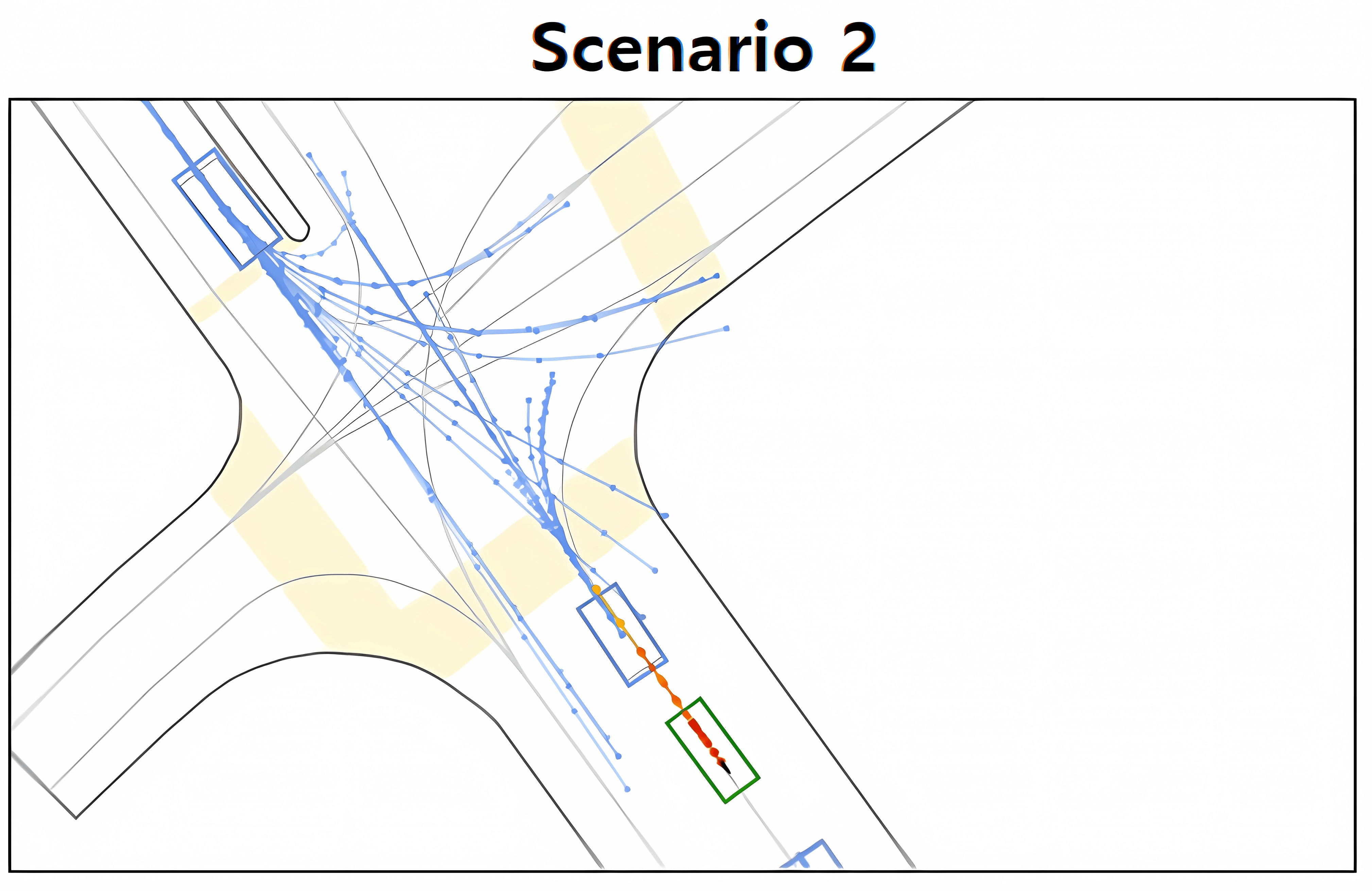
In scenario 2, a clear observation here is the overlapping and intersecting trajectories, especially around the intersection. These trajectories seem to be “blurred” between the lanes rather than being clearly defined in one lane or another. While in the scenario 3, despite the clearer trajectory forecasts than the previous one, we can still observe “mode blur” problems. Some predicted trajectories seem to be dispersed across the lane without a distinct path.
This issue can lead to the Autonomous Vehicle (AV) having to make frequent adjustments to its path. This is indeed problematic as the AV might need to execute sudden brakes and make abrupt steering changes. This not only results in an uncomfortable ride for the passengers but also raises safety concerns.
Reason Why “Mode Blur” Happens
The reason for this problem is the use of Variational Autoencoders (VAEs) in the trajectory forecasting models since they have a well-known limitation: the outputs that they generate can often be “blurry”. The authors of paper [1] observed that similar problem also found in the trajectory planning case, not only in the tasks involving image reconstruction and synthesis.
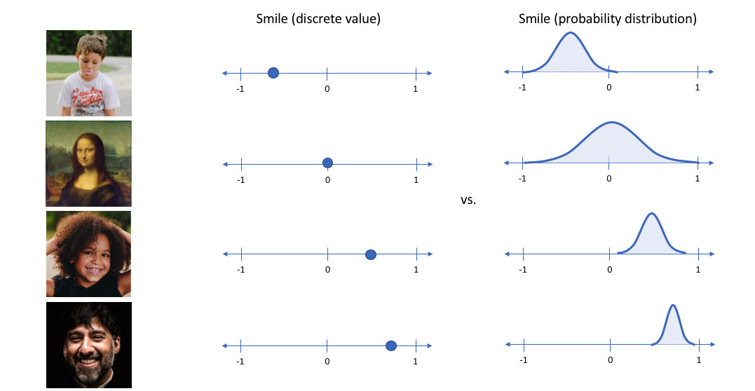
VAEs aim to learn a probabilistic latent space representation of the data. So instead of generating fixed value of latent variable, what VAE does is to learn the latent space distribution and sample from it in order to get the latent vector that can be used to reconstruct the input.
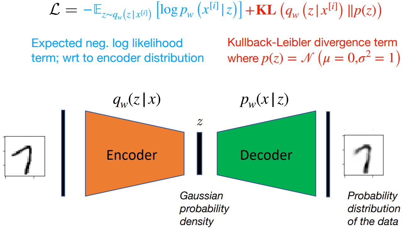
The main objective of the VAEs is to optimize the Evidence Lower Bound Objective (ELBO) on the marginal likelihood of data \(p_\theta(\mathbf{x})\). This lower bound is formulated as:
\[\text{ELBO} = \mathbb{E}_{q_\phi(\mathbf{z} \mid \mathbf{x})}[\log p_\theta(\mathbf{x} \mid \mathbf{z})] - D_{KL}(q_\phi(\mathbf{z}|\mathbf{x}) \| p_\theta(\mathbf{z}))\]Two components in the ELBO:
- The first term \(\mathbb{E}_{q_\phi(\mathbf{z} \mid \mathbf{x})}[\log p_\theta(\mathbf{x} \mid \mathbf{z})]\) is the reconstruction loss which measures how well the VAE reconstructs the original data when sampled from the approximate posterior \(q_\phi\).
- The second term \(D_{KL}(q_\phi(\mathbf{z} \mid \mathbf{x}) \| p_\theta(\mathbf{z}))\) is the Kullback-Leibler divergence between the approximate posterior \(q_\phi\) and the prior \(p_\theta\). This term acts as a regularizer, pushing the approximate posterior towards the prior.
For more detailed understanding, you can take a look at this very good blogpost Lil’Log or excellent explanation by Ahlad Kumar.
As far as i know, several previous works assume the prior distribution for the latent variables, \(Z\), to be a standard Gaussian distribution, \(\mathcal{N}(0, I)\), which is fixed and does not depend on the input context. The reason for using this assumption is to simplify the learning process.
This can be problematic because a standard Gaussian prior assumes that the latent space is unimodal and therefore does not fully capture the multi-modal nature of the future trajectories where multiple distinct future paths (modes) are possible. This will make the alignment via KL divergence much more difficult for the model.
Furthermore, when the VAE learns to represent data in the latent space, it must balance the reconstruction and KL divergence terms. It wants to spread out the representations to minimize the reconstruction loss (since the trajectory distribution is multi-modal) but it is also constrained by the KL divergence to keep these representations from getting too dispersed (since the prior is assumed to be unimodal).
As a consequence, during the generation phase, when the model samples from these latent representations, it also may end up sampling from “in-between” spaces if the distinct modes are not well-separated.
So in this case, the “mode blur” problem is most likely happened due to the balancing act between reconstruction loss and the KL divergence done by the ELBO objective function. When generating data, the VAE may generate a predicted trajectory that doesn’t clearly commit to any of the possible paths. Instead, it generates a trajectory that lies somewhere in between.
Key Contributions
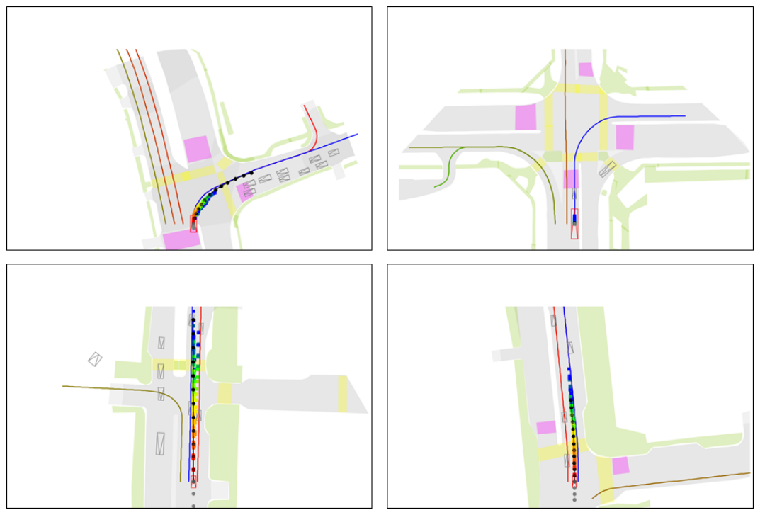
Based on my understanding so far, there are 4 major contributions of this paper [1]:
-
Mitigating Mode Blur: Propose a hierarchical latent structure within a VAE-based forecasting model to avoid “mode blur” problem, enabling clearer and more precise trajectory predictions.
-
Context Vectors: Two lane-level context vectors
VLIandV2Iare conditioned on the low-level latent variables for more accurate trajectory predictions. -
Additional Methods: Introduce positional data preprocessing and GAN-based regularization to further enhance the performance.
-
Benchmark Performance: The state-of-the-art performance on two large-scale real-world datasets.
Hierarchical Latent Structure (HLS)
Introduction to HLS
You may wonder how that kind of approach can avoid the “mode blur” problem that happens in the previous work. Basically they implement Conditional-VAE with the input \(\mathbf{X}_{i}\) and \(\mathcal{C}_{i}\) as conditional variable. The goal of the proposed method is to generate a trajectory distribution \(p\left(\mathbf{Y}_{i} \mid \mathbf{X}_{i}, \mathcal{C}_{i}\right)\) for vehicles.
The generated trajectory distribution is represented as a sum of modes, weighted by their probability or importance. Mathematically, it can be defined like below :
\[p\left(\mathbf{Y}_{i} \mid \mathbf{X}_{i}, \mathcal{C}_{i}\right)=\sum_{m=1}^{M} \underbrace{p\left(\mathbf{Y}_{i} \mid E_{m}, \mathbf{X}_{i}, \mathcal{C}_{i}\right)}_{\text {mode }} \underbrace{p\left(E_{m} \mid \mathbf{X}_{i}, \mathcal{C}_{i}\right)}_{\text {weight }}\]Note that the term “mode” represents a plausible path, and the term “weight” represents the probability of each mode occurring.
HLS to Avoid “Mode Blur”
The paper assumes that the trajectory distribution can be approximated as a mixture of simpler distributions. Each of these simpler distributions, or “modes”, represents a distinct pattern or type of trajectory that a vehicle could follow.
The key intuition here is that instead of learning the overall distributions of the future trajectories, the proposed method tries to consider each possible trajectory (mode) separately and then approximate the trajectory distributions by combining all possible modes with its own probability.
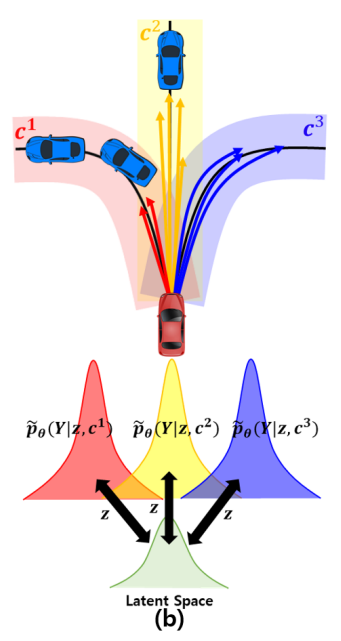
To capture this mixture of distributions, the HLS model employs two levels of latent variables:
- Low-level latent variable \(\mathbf{z}_{l}\): Used to model individual modes of the trajectory distributions.
- High-level latent variable \(\mathbf{z}_{h}\): Employed to determine the weights for different modes.
The mathematical equation of the new objective function can be expressed as below :
\[\begin{aligned} \mathcal{L}_{ELBO} = & -\mathbb{E}_{\mathbf{z}_{l} \sim q_{\phi}}\left[\log p_{\theta}\left(\mathbf{Y}_{i} \mid \mathbf{z}_{l}, \mathbf{X}_{i}, \mathcal{C}_{i}^{m}\right)\right] \\ & + \beta KL\Big(q_{\phi}\left(\mathbf{z}_{l} \mid \mathbf{Y}_{i}, \mathbf{X}_{i}, \mathcal{C}_{i}^{m}\right)\| p_{\gamma}\left(\mathbf{z}_{l} \mid \mathbf{X}_{i}, \mathcal{C}_{i}^{m}\right)\Big), \end{aligned}\]The key aspect here is that the prior \(p_{\gamma}(\mathbf{z}_l \mid \mathbf{X}_{i}, \mathcal{C}_{i}^{m})\) is conditional on the input and the context. This implies that the model isn’t learning a single static prior for all data but rather a dynamic prior that adapts based on the specific input \(\mathbf{X}_i\) and context \(\mathcal{C}_{i}^{m}\).
This conditionality allows the model to learn different representations for different subsets of data, guided by the vehicle’s past trajectory and additional scene information relevant to the vehicle. By doing so, the model can capture the nuances and variations in trajectory distributions that are specific to different traffic situations and lane configurations.
That means we can have much more richer variations in the prior distribution which hopefully can reduce the gap that can happen between it and the posterior distribution (since it is conditioned on the trajectory distributions that are known to be multi-modal).
By structuring the model in this way, the HLS method can generate trajectory predictions that are a combination of distinct, plausible paths that a vehicle might realistically take, each with its own probability.
Generating VLI and V2I Context Vectors
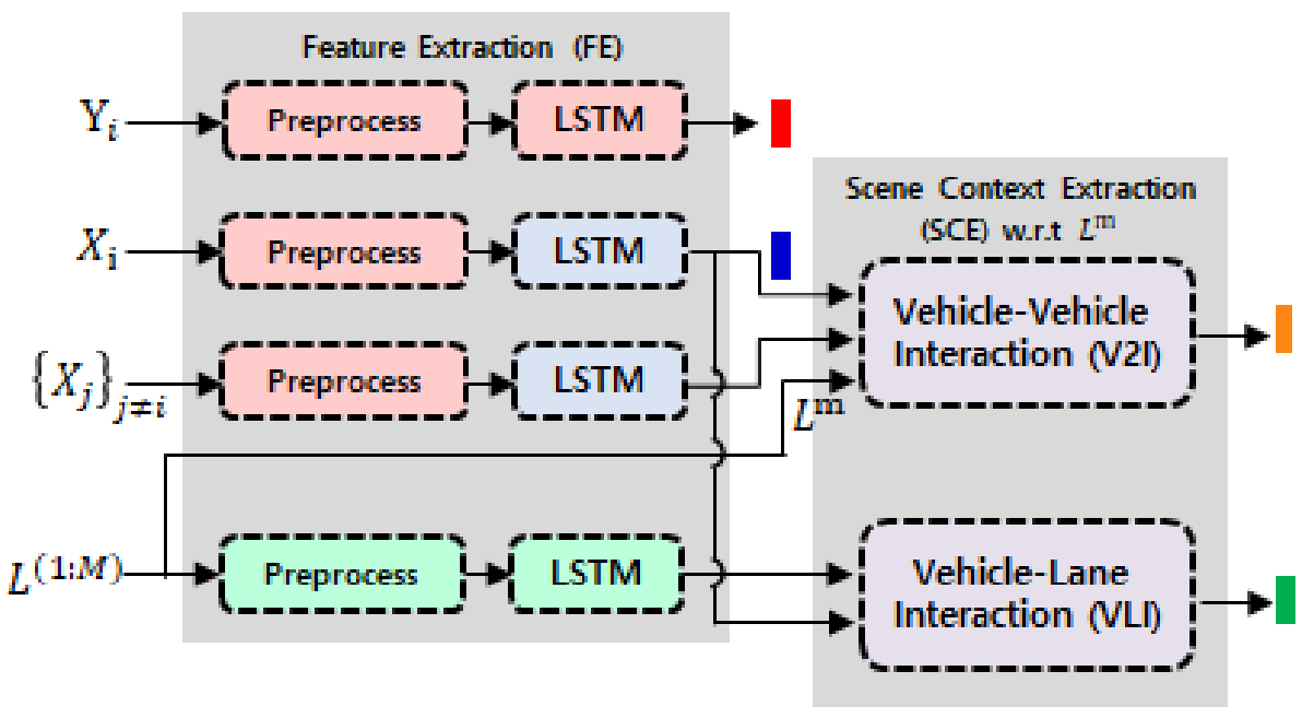
Now, we will discuss how the VLI and V2I context vectors are generated in the HLS paper. This process is done in the Scene Context Extraction module of the proposed trajectory forecasting model:
VLI Context Vector:
The VLI context vector, denoted as \(\mathbf{a}_{i}^{m}\), is built around the idea that a vehicle’s trajectory is influenced by its reference lane (\(\mathbf{L}^{m}\)) and the surrounding lanes. The model first identifies the reference lane for the vehicle \(V_{i}\) and then calculates weights (\(\alpha_{l}\)) for the surrounding lanes. These weights signify the relative importance of each surrounding lane compared to the reference lane.
The weights (\(\alpha_{l}\)) are determined through an attention mechanism between \(\tilde{\mathbf{X}}_{i}\) and \(\tilde{\mathbf{L}}^{(1: M)}\). The attention operation assesses how relevant each surrounding lane is in the context of the vehicle’s past motion and the current trajectory.
Then, the final VLI context vector is a concatenation of the encoded reference lane \(\tilde{\mathbf{L}}^{m}\) and a weighted sum of the encoded surrounding lanes, where the weights are the attention scores \(\alpha_{l}\).
The final mathematical expression for generating VLI context vector can be written :
V2I Context Vector:
The V2I context vector, denoted as \(\mathbf{b}_{i}^{m}\), captures the interactions between the vehicle \(V_{i}\) and its neighboring vehicles within a certain distance (defined by a threshold \(\tau\)). This subset of neighboring vehicles is represented by \(\mathcal{N}_{i}^{m}\).
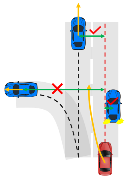
The interactions itself are modeled using a Graph Neural Network (GNN). Message passing occurs from each neighboring vehicle \(V_{j}\) to the vehicle \(V_{i}\), defined by \(\mathbf{m}_{j \rightarrow i}\). These messages are a function of the relative positions and hidden states of \(V_{i}\) and \(V_{j}\) at each time step, processed through a Multi-Layer Perceptron (MLP).
Then, the messages are aggregated, and the aggregated output is fed into a Gated Recurrent Unit (GRU) to update the hidden state of \(V_{i}\). The process repeats for \(K\) rounds, capturing the evolving interaction over time.
Finally, the V2I context vector is the sum of the final hidden states of all neighboring vehicles, representing the cumulative effect of the vehicle-vehicle interactions on \(V_{i}\)’s future trajectory.
HLS Overall Architecture
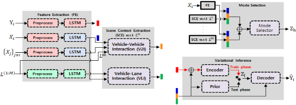
Encoder, Prior, and Decoder:
-
Encoder: Approximate the posterior distributions with Multi-Layer Perceptrons (MLPs) where the encoding \(\tilde{\mathbf{Y}}_{i}\) and \(\mathbf{c}_{i}^{m}\) become inputs. Thus, it outputs two vectors, mean \(\mu_{e}\) and standard deviation \(\sigma_{e}\). Notably, the encoder is used only during the training phase because \(\mathbf{Y}_{i}\) is not available during inference.
-
Prior: Represents the prior distribution over the latent variable and is also implemented as MLPs. It takes \(\mathbf{c}_{i}^{m}\) as its input and outputs mean \(\mu_{p}\) and standard deviation \(\sigma_{p}\) vectors.
-
Decoder: Generates \(\hat{\mathbf{Y}}_{i}\) via an LSTM network. The input consists of an embedding of the predicted position \(\mathbf{e}_{i}^{t}\) along with \(\mathbf{c}_{i}^{m}\) and \(\mathbf{z}_{l}\). The LSTM updates its \(\mathbf{h}_{i}^{t+1}\) based on these inputs, and the new predicted position \(\hat{\mathbf{p}}_{i}^{t+1}\) is generated from this hidden state.
Note that the lane-level scene context vector is just the concatenation of
\[\mathbf{c}_{i}^{m}=\left[\tilde{\mathbf{X}}_{i} ; \mathbf{a}_{i}^{m} ; \mathbf{b}_{i}^{m}\right]\]The design of this method aims to provide a holistic understanding of the vehicle’s motion by considering both lane and vehicle interactions. Lanes guide the general direction of movement, while nearby vehicles influence more immediate decisions like lane changes or speed adjustments.
Conclusion
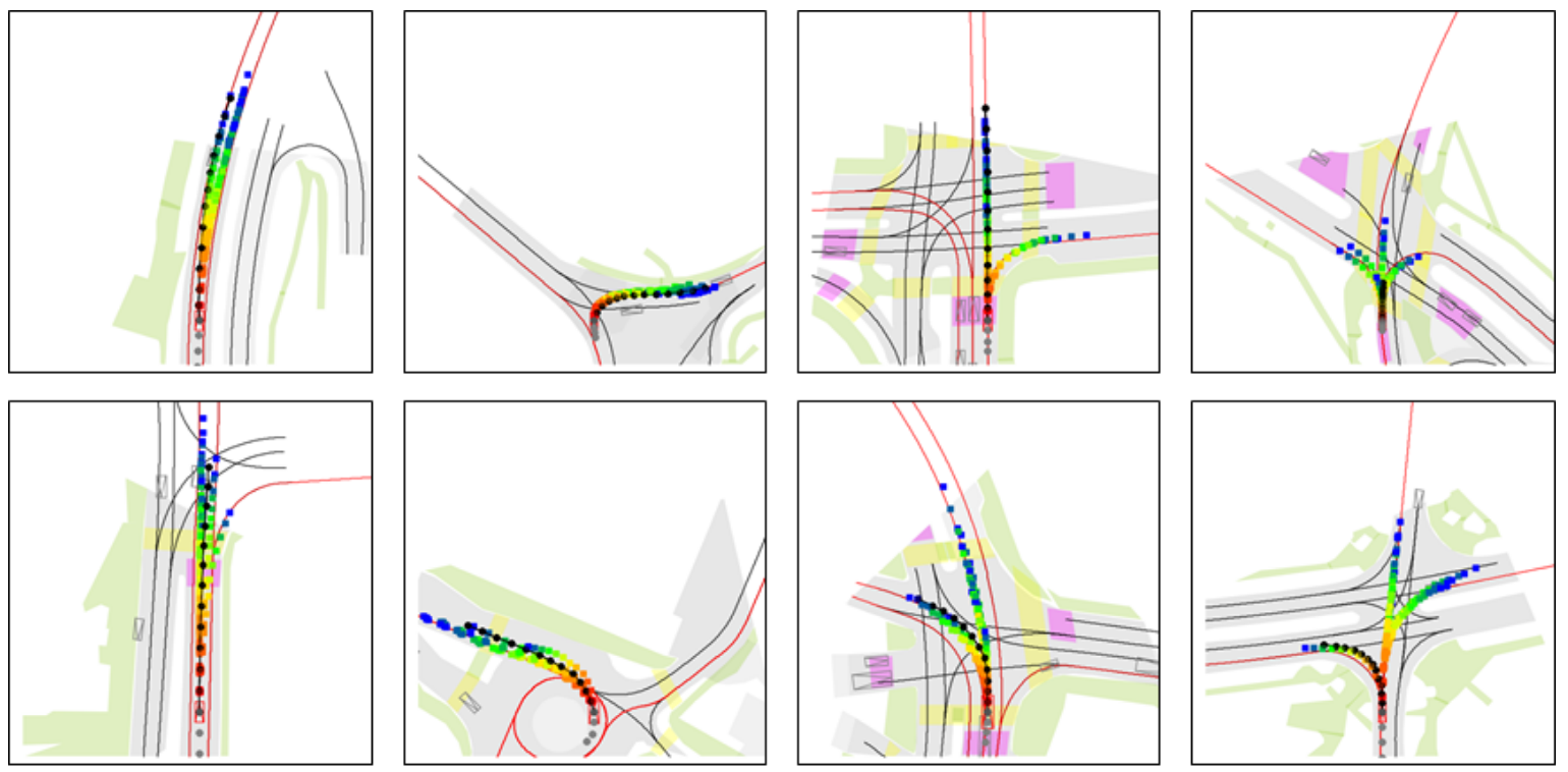
This paper proposes a novel and unique way to tackle the problem of “mode blur” predictions in trajectory forecasting. Instead of assuming the prior as simple unimodal distribution, it uses conditional-VAE to capture richness and diversity of the future trajectories which is a multi-modal distribution. The final future trajectories are combinations of all possible modes each with its weight. The use of lane-level context vectors can add more precision, especially in understanding vehicle-lane and vehicle-vehicle interactions. This work not only sharpens the predictions but also can outperform the previous SOTA models in terms of accuracy.
References
- Hierarchical Latent Structure for Multi-Modal Vehicle Trajectory ForecastingEuropean Conference on Computer Vision (ECCV), 2022
- LookOut: Diverse Multi-Future Prediction and Planning for Self-DrivingInternational Conference on Computer Vision (ICCV), 2021