What are JAX and Flax? Why those Deep Learning Frameworks can be Very Important?
Understanding JAX and Flax!
Hello, everyone! Today, we will learn about two powerful tools for machine learning: JAX and Flax. These frameworks can be much faster than the common deep learning frameworks, such as Pytorch and Tensorflow. JAX can help us with fast math calculations, and Flax can make it easier to build neural networks. We’ll use both to make a simple image classifier for handwritten digits.

Table of Contents
- Introduction
- So, Why Using JAX and Flax?
- What You’ll Learn
- JAX and Flax Implementation w/ MNIST Image Classification
Introduction
Before diving into the technical details, let’s discuss why we even need frameworks like JAX and Flax when we already have powerful libraries like PyTorch and TensorFlow.
What’s the Issue with Existing Frameworks?
Don’t get me wrong—PyTorch and TensorFlow are great. They are powerful, easy to use, and have huge communities. However, they can be a bit rigid for some research needs:
- Not So Easy to Customize: If you need to modify the behavior of the training loop or gradient calculations, you might find it challenging.
- Debugging: Debugging can be hard, especially when computation graphs become complex.
So, Why Using JAX and Flax?
JAX is like NumPy which means that JAX’s features is its NumPy-compatible API allowing for easy transition from NumPy to JAX for numerical operations, but supercharged:
- Flexibility: JAX is functional and allows for more fine-grained control, making it highly customizable.
- Performance: With its just-in-time compilation, JAX can optimize your code for high-speed numerical computing.
In many cases, it would make sense to use jax.numpy (often imported as jnp) instead of ordinary NumPy to take advantage of JAX’s features like automatic differentiation and GPU acceleration.
Why Flax?
Flax is like the cherry on top of JAX:
- Simplicity: Building neural networks becomes straightforward.
- Extendable: Designed with research in mind, you can easily add unconventional elements to your network or training loop.
What You’ll Learn
- What are JAX and Flax?
- How to install them
- Building a simple CNN model for MNIST image classification
What is JAX?
JAX is a library that helps us do fast numerical operations. It can automatically make our code run faster and allows us to use the GPU easily by utilizing Just-In-Time (JIT) Compilation. It is widely used in research for its flexibility and speed.
So, what is Just-In-Time Compilation?
Imagine you’re a chef, and you have a recipe (your code). Traditional Python executes this recipe step-by-step, which is time-consuming. JIT compilation is like having an assistant chef who learns from watching you and then can perform the entire recipe in a much more optimized manner.
In my experience, after applying JIT compilation properly, JAX can outperform TensorFlow and Pytorch in training speed, making it highly efficient for machine learning tasks.
While JAX is powerful, it also requires careful coding practices. For example, to take full benefits of using JIT compilation, it is crucial to avoid changing the code inside the training loop to prevent re-compilation, which can slow down the training process. Once you grasp these nuances, harnessing JAX’s full power becomes straightforward.
What is Flax?
Flax is built on top of JAX and provides a simple way to build and train neural networks. It is designed to be flexible, making it a good choice for research projects.
JAX and Flax w/ MNIST Image Classification
Let’s go into simple practical implementation on MNIST dataset. MNIST Image Classification is a simple but fundamental task in machine learning. It gives us a perfect playground to explore JAX and Flax without getting lost in the complexity of the task itself.
Installing JAX and Flax
First, let’s install JAX and Flax. Open your terminal and run:
pip install --upgrade jax jaxlib
pip install flax
Import Libraries
Let’s import all the libraries we need.
import jax
import flax
import jax.numpy as jnp
from flax import linen as nn
from jax import random
from tensorflow.keras import datasets
Prepare the Data
We’ll use the MNIST dataset, which is a set of 28x28 grayscale images of handwritten digits. We normalize the images by dividing by 255, as this scales the pixel values between 0 and 1, which generally helps the model to learn more efficiently.
(train_images, train_labels), (test_images, test_labels) = datasets.mnist.load_data()

# Normalize and reshape the data using JAX's NumPy
train_images = jnp.expand_dims(train_images / 255.0, axis=-1).astype(jnp.float32)
test_images = jnp.expand_dims(test_images / 255.0, axis=-1).astype(jnp.float32)
Create the Model
Now let’s build a simple Convolutional Neural Network (CNN) using Flax.
# Define the CNN model using Flax
class CNN(nn.Module):
    """
    A simple CNN model for MNIST classification.
    """
    @nn.compact
    def __call__(self, x: jnp.ndarray) -> jnp.ndarray:
        x = nn.Conv(features=32, kernel_size=(3, 3))(x)
        x = nn.relu(x)
        x = nn.avg_pool(x, window_shape=(2, 2), strides=(2, 2))
        x = nn.Conv(features=64, kernel_size=(3, 3))(x)
        x = nn.relu(x)
        x = nn.avg_pool(x, window_shape=(2, 2), strides=(2, 2))
        x = x.reshape((x.shape[0], -1))
        x = nn.Dense(features=256)(x)
        x = nn.relu(x)
        x = nn.Dense(features=10)(x)
        return nn.log_softmax(x)
Initialize the Model
Before using our model, we need to initialize it. Initialization is crucial because it sets the initial random weights of the model, which will be updated during training.
key = random.PRNGKey(0)
model = CNN()
x = jnp.ones((1, 28, 28, 1), jnp.float32)
params = model.init(key, x)
Training
Now, let’s train the model. But first, let’s initialize the optimizer. We will use the Adam optimizer provided by Optax. Optax is a flexible and extensible optimization library that provides a wide range of optimization algorithms.
# Initialize the optimizer
import optax
optimizer = optax.adam(0.001)
opt_state = optimizer.init(params)
We won’t go into detail about training loops here, but you can use JAX’s grad function to compute gradients and update the model weights. We use JAX’s jit function to compile the train_step function, speeding up our training loop. Just-In-Time (JIT) compilation improves the performance by compiling Python functions to optimized machine code at runtime.
from jax import grad, jit, value_and_grad
from jax.scipy.special import logsumexp

def loss_fn(params: dict, images: jnp.ndarray, labels: jnp.ndarray) -> float:
    """
    Computes the loss between the predicted labels and true labels.
    """
    logits = CNN().apply(params, images)
    logprobs = logits - logsumexp(logits, axis=-1, keepdims=True)
    return -jnp.mean(jnp.sum(logprobs * labels, axis=-1))

@jit
def train_step(opt_state: optax.OptState, params: dict, images: jnp.ndarray, labels: jnp.ndarray) -> tuple:
    """
    Performs a single training step.
    """
    loss, grads = value_and_grad(loss_fn)(params, images, labels)
    updates, new_opt_state = optimizer.update(grads, opt_state)
    new_params = optax.apply_updates(params, updates)
    return new_opt_state, new_params, loss
Pre-Compiling Functions for Faster Execution
You might have noticed a somewhat unusual block of code right before our training loop:
# Pre-compile functions
# Use a small subset of data to trigger JIT compilation
sample_images = jnp.ones((1, 28, 28, 1), jnp.float32)
sample_labels = jnp.zeros((1, 10), jnp.float32)
jit_loss_fn = jit(loss_fn)
jit_train_step = jit(train_step)

# Trigger JIT compilation
_ = jit_loss_fn(params, sample_images, sample_labels)
_ = jit_train_step(opt_state, params, sample_images, sample_labels)
What’s going on with the code above? This block of code is a technique to “warm up” or pre-compile our JAX functions, so they run faster during our training loop.
We also create a small subset of dummy data, sample_images and sample_labels, that matches the shape and type of our real data. Then, we use JAX’s jit function to indicate that loss_fn and train_step should be JIT compiled.
Finally, we run these JIT-compiled functions once using our dummy data. This step is crucial as it triggers the JIT compilation process, converting our Python functions into highly optimized machine code.
Why Do We Need This?
JAX uses Just-In-Time (JIT) compilation to optimize our code. JIT compilation works by looking at the operations in our functions and creating an optimized version of these functions. However, JIT compilation itself takes time. By pre-compiling, we do this step before entering our training loop, ensuring that our code runs at maximum speed when it matters the most.
This pre-compilation step is particularly helpful in scenarios where the training loop has to run multiple times, helping us save time in the long run.
Next, let’s divide the training data into training and validation sets:
from sklearn.model_selection import train_test_split

# Split the training data into training and validation sets
train_images, val_images, train_labels, val_labels = train_test_split(train_images, train_labels, test_size=0.2, random_state=42)

# One-hot encode labels
train_labels_onehot = jax.nn.one_hot(train_labels, 10)
val_labels_onehot = jax.nn.one_hot(val_labels, 10)
Now we can write the training loop.
import pickle
import time

start_time = time.time()

# Initialize variables to keep track of best model and performance
best_val_loss = float('inf')
best_params = None

# Lists to keep track of loss values for plotting
train_losses = []
val_losses = []

for epoch in range(num_epochs):
    # Training loop
    train_loss_epoch = []
    for i in range(0, len(train_images), batch_size):
        batch_images = jnp.array(train_images[i:i + batch_size])
        batch_labels = jnp.array(train_labels_onehot[i:i + batch_size])
        opt_state, params, loss = train_step(opt_state, params, batch_images, batch_labels)
        train_loss_epoch.append(loss)

    avg_train_loss = jnp.mean(jnp.array(train_loss_epoch))
    train_losses.append(avg_train_loss)

    # Validation loop
    val_loss_epoch = []
    for i in range(0, len(val_images), batch_size):
        batch_images = jnp.array(val_images[i:i + batch_size])
        batch_labels = jnp.array(val_labels_onehot[i:i + batch_size])
        val_loss = loss_fn(params, batch_images, batch_labels)
        val_loss_epoch.append(val_loss)

    avg_val_loss = jnp.mean(jnp.array(val_loss_epoch))
    val_losses.append(avg_val_loss)

    print(f"Epoch {epoch + 1}, Train Loss: {avg_train_loss}, Val Loss: {avg_val_loss}")

    # Save best model
    if avg_val_loss < best_val_loss:
        best_val_loss = avg_val_loss
        best_params = params

# Calculate the training time with JAX
end_time = time.time()
jax_training_time = end_time - start_time
print(f"Training time with JAX: {jax_training_time:.4f} seconds")

# Save the best model parameters to a file
with open('best_model_params.pkl', 'wb') as f:
    pickle.dump(best_params, f)
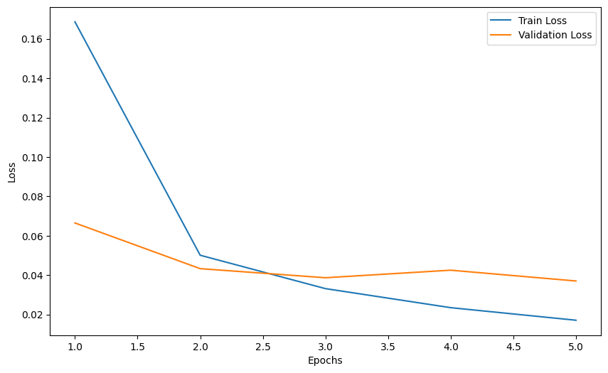
Then, we can plot the training and validation loss like below:
import matplotlib.pyplot as plt
plt.figure(figsize=(10, 6))
plt.plot(range(1, num_epochs + 1), train_losses, label='Train Loss')
plt.plot(range(1, num_epochs + 1), val_losses, label='Validation Loss')
plt.xlabel('Epochs')
plt.ylabel('Loss')
plt.legend()
plt.show()

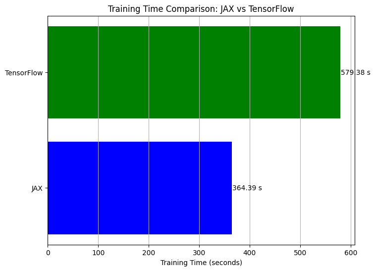
And that’s it! You’ve built a simple CNN for MNIST digit classification using JAX and Flax. Now, to get the point on why using those frameworks can be really crucial, let’s compare its training time with the training time when using tensorflow. Note that we measured the time taken to train a Convolutional Neural Network (CNN) on the MNIST dataset using both JAX and TensorFlow.
Also note that for fair comparison, both models have the same architecture and are trained for the same number of epochs and batch size.
import tensorflow as tf
from tensorflow.keras import layers, models

# Preparing data
(train_images, train_labels), (val_images, val_labels) = datasets.mnist.load_data()
train_images = train_images.reshape((60000, 28, 28, 1)).astype('float32') / 255
val_images = val_images.reshape((10000, 28, 28, 1)).astype('float32') / 255

train_labels = tf.keras.utils.to_categorical(train_labels, 10)
val_labels = tf.keras.utils.to_categorical(val_labels, 10)

# Creating the model
model = models.Sequential([
    layers.Conv2D(32, (3, 3), activation='relu', input_shape=(28, 28, 1)),
    layers.AveragePooling2D((2, 2)),
    layers.Conv2D(64, (3, 3), activation='relu'),
    layers.AveragePooling2D((2, 2)),
    layers.Flatten(),
    layers.Dense(256, activation='relu'),
    layers.Dense(10, activation='softmax')
])

# Compiling the model
model.compile(optimizer='adam',
              loss='categorical_crossentropy',
              metrics=['accuracy'])

# Measuring time for training
start_time = time.time()

# Fitting the model
history = model.fit(
    train_images, train_labels,
    epochs=10,
    batch_size=64,
    validation_data=(val_images, val_labels)
)

end_time = time.time()

non_jax_training_time = end_time - start_time

print(f"Training time without JAX: {non_jax_training_time:.4f} seconds")
In machine learning, training time is a crucial factor. Faster training allows for more iterations and experiments, speeding up the development process. Below is a bar graph that shows the training time for each framework.
# Labels and corresponding values
labels = ['JAX', 'TensorFlow']
times = [jax_training_time, non_jax_training_time]

# Create the bar chart
plt.figure(figsize=(8, 6))
plt.barh(labels, times, color=['blue', 'green'])
plt.xlabel('Training Time (seconds)')
plt.title('Training Time Comparison: JAX vs TensorFlow')
plt.grid(axis='x')

# Annotate with the exact times
for i, time in enumerate(times):
    plt.text(time + 1, i, f'{time:.2f} s', va='center')

plt.show()

As you can see, using JAX in simple dataset like MNIST can increase the speed significantly. You can imagine how fast it is when implementing it in bigger datasets and much more complex tasks!!
Conclusion
JAX and Flax are powerful tools for machine learning research and projects. JAX provides fast and flexible numerical operations, while Flax offers a simple and extendable way to build neural networks.
I hope this post helps you understand the basics of JAX and Flax. Below I also attach runned jupyter notebook about this blogpost. Happy coding!