Grad-CAM Demystified, Understanding the Magic Behind Visual Explanations in Neural Networks
Introduction
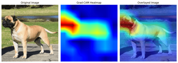
Convolutional Neural Networks (CNNs) are amazing. They can recognize cats in pictures, help self-driving cars see, and even beat humans at games. But what most people see about neural networks is this, they’re like magic boxes: data goes in, and the answer comes out, without knowing what happens in between. So, how do we know what part of an image the network finds important for its decision? Introducing Grad-CAM method, a technique that helps us “see” what the network is looking at.

What is Grad-CAM?
Grad-CAM stands for Gradient-weighted Class Activation Mapping. Why the name is like that? In short, we use gradient to help us understand how neural networks behave in certain circumstances, while activation here is analogous with the level of excitement or interest the neural network has when it comes to certain features used in recognizing the important part in the image (we will discuss in detail about it later). How it does that? Basically, Grad-CAM will create what we call a “heatmap.” Imagine you have your cat picture. Now, think of putting a see-through red paper over it. This red paper will have some areas darker and some areas lighter. The darker areas show where the neural network looked the most. Maybe the network looked a lot at the cat’s eyes and a little at the tail. This heatmap will help you “see” what parts of the picture made the neural network decide it’s looking at a cat. It’s like the network is saying, “Look, I think this is a cat because of these parts of the picture.”
The Core Idea
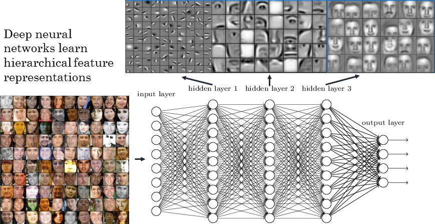
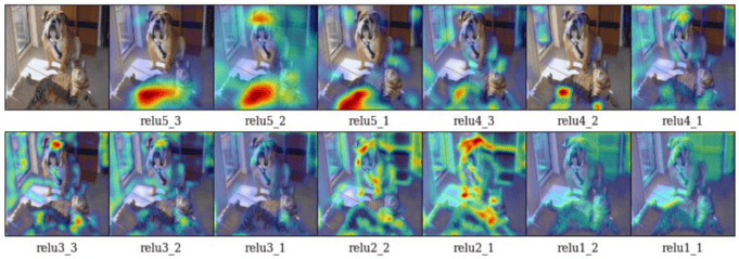
Grad-CAM will use something called “gradients” which can tell us how much each neuron’s activity would need to change in order to affect the final decision (class scores or logits that are output by the neural network) of the model. The key intuition here is that if the gradient is large in magnitude, a small change in the neuron’s activity will have a significant impact on the final decision. Conversely, if the gradient is small, the neuron’s contribution to the final decision is relatively minor. Grad-CAM also often uses deeper layers in order to visualize important part of the image. In a CNN, the early layers usually can only understand simple things like edges or colors. The deeper you go, the more complex the things they understand, like ears or whiskers. Grad-CAM focuses on the last set of these layers because they understand both the important details (like whiskers) and the bigger picture (like the shape of a cat). Remember that in the context of CNN, feature maps in the early layers of can only capture basic features like edges and textures. But, as you move deeper into the network, the feature maps begin to assemble these into more complex structures, capturing higher-level features like shapes, patterns, and even entire objects in some cases.
How Does it Work in Quite Detail?
Step 1: Backward Pass
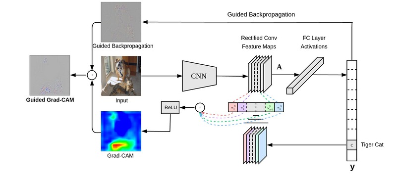
First, we need to find out how much each part of our image contributed to the final decision. So, we go backward through the network, from the output (“this is a cat”) toward the input image. As we go back, we calculate something called gradients. Remember that the “gradient” of a neuron with respect to the final decision can give us a measure of sensitivity. Specifically, it tells us how much the final output (e.g., the probability score for the class “cat”) would change if the activity of that particular neuron were to change by a small amount. In mathematical terms, if \(y\) is the final output and \(A_{ij}^k\) is the activation of neuron \(k\) at position \((i, j)\) in some layer, then \(\frac{\partial y}{\partial A_{ij}^k}\) is the gradient that tells us the rate of change of \(y\) with respect to \(A_{ij}^k\).
Step 2: Average Pooling
We then average these gradients across the spatial dimensions (width and height) of each feature map. This gives us a single number for each feature map, which we call the “importance weight.”
The math looks like this:
\[\alpha_{k}^{c} = \frac{1}{Z} \sum_{i} \sum_{j} \frac{\partial y^{c}}{\partial A_{i j}^{k}}\]Here, \(\alpha_{k}^{c}\) is the importance weight for feature map \(k\) when identifying class \(c\).
Step 3: Weighted Sum
Next, we take a weighted sum of our original feature maps, using these importance weights. This gives us a rough heatmap. We will explain that in more detail about how it is used in the step 5.
\[L_{\text{Grad-CAM}}^{c} = \text{ReLU}\left(\sum_{k} \alpha_{k}^{c} A^{k}\right)\]Step 4: ReLU Activation
Finally, we apply a ReLU (Rectified Linear Unit) function to this heatmap. Why? Because we’re only interested in the parts of the image that positively influence the final decision.
Step 5: Understanding the Heatmap
At this point, you might wonder, “How exactly does the weighted sum of feature maps and ReLU activation contribute to generating a heatmap?”
The heatmap \(L_{\text{Grad-CAM}}^{c}\) is essentially a 2D spatial map of the image that highlights the important regions, which have been “weighted” based on their contribution to the class score. Recall that this weighted sum can be formally represented as:
\[L_{\text{Grad-CAM}}^{c} = \text{ReLU}\left(\sum_{k} \alpha_{k}^{c} A^{k}\right)\]Here, \(\alpha_{k}^{c}\) serves as a weight indicating the importance of feature map \(A^{k}\) for the particular class \(c\). So, when we multiply \(\alpha_{k}^{c}\) with the feature map \(A^{k}\), we’re essentially weighing the feature map based on its importance for class \(c\).
After the weighted sum, we apply the ReLU non-linearity function. Why ReLU? This is to ensure that only the features that have a positive influence on the class of interest are kept. ReLU zeroes out negative values, leaving only the positive regions that are important for identifying the specific class. The ReLU function can be represented mathematically as:
\[\text{ReLU}(x) = \max(0, x)\]Thus, the heatmap generated is a filtered version of the weighted sum of feature maps, where only the ‘positively contributing’ features are illuminated. This enables you to see which regions in the image were pivotal in making the final class decision.
A Simple PyTorch Grad-CAM Implementation
To see Grad-CAM in action, let’s walk through a straightforward example using PyTorch. We’ll use a pretrained VGG16 model for this demonstration.
First, make sure to install PyTorch if you haven’t already.
pip install torch torchvision
Import Libraries
import torch
import torch.nn as nn
import torchvision.models as models
import torchvision.transforms as transforms
from PIL import Image
Load Pretrained Model
# Load a pretrained VGG16 model
model = models.vgg16(pretrained=True)
model.eval()
Utility Function to Get Model Features and Gradients
from typing import Tuple

def get_features_gradients(model: nn.Module, x: torch.Tensor) -> Tuple[torch.Tensor, torch.Tensor]:
    """
    Forward pass to get the features and register hook to get gradients.

    Parameters:
    - model (nn.Module): Neural network model
    - x (torch.Tensor): Input image tensor

    Returns:
    - features (torch.Tensor): Extracted features from the last convolutional layer
    - gradients (torch.Tensor): Gradients w.r.t the features
    """
    features = None
    gradients = None

    def hook_feature(module, input, output):
        nonlocal features
        features = output.detach()

    def hook_gradient(module, grad_input, grad_output):
        nonlocal gradients
        gradients = grad_output[0].detach()

    # Register hooks
    handle_forward = model.features[-1].register_forward_hook(hook_feature)
    handle_backward = model.features[-1].register_backward_hook(hook_gradient)

    # Forward and backward pass
    model.zero_grad()
    output = model(x)
    # Class-specific backprop
    output.backward(torch.Tensor([[1 if idx == 243 else 0 for idx in range(output.shape[1])]]))

    # Remove hooks
    handle_forward.remove()
    handle_backward.remove()

    return features, gradients
Generate Grad-CAM Heatmap
from typing import Tuple

def generate_grad_cam(features: torch.Tensor, gradients: torch.Tensor, image_shape: Tuple[int, int]) -> torch.Tensor:
    """
    Generate Grad-CAM heatmap.

    Parameters:
    - features (torch.Tensor): Extracted features from the last convolutional layer
    - gradients (torch.Tensor): Gradients w.r.t the features
    - image_shape (Tuple[int, int]): Original shape of the input image (height, width)

    Returns:
    - torch.Tensor: Grad-CAM heatmap
    """
    # Global average pooling on gradients to get neuron importance
    alpha = gradients.mean(dim=[2, 3], keepdim=True)

    # Weighted sum of feature maps based on neuron importance
    weighted_features = features * alpha

    # ReLU applied on weighted combination of feature maps
    heatmap = nn.functional.relu(weighted_features.sum(dim=1, keepdim=True))

    # Resizing the heatmap to original image size
    heatmap = nn.functional.interpolate(heatmap, size=image_shape, mode='bilinear', align_corners=False)

    return heatmap
Function to Overlay Heatmap on Original Image
import cv2
import matplotlib.pyplot as plt
from typing import Union
import numpy as np

def overlay_heatmap_on_image(image: Union[np.ndarray, Image.Image],
                             heatmap: Union[np.ndarray, torch.Tensor],
                             alpha: float = 0.5) -> np.ndarray:
    """
    Overlay the Grad-CAM heatmap on the original image.

    Parameters:
    - image (np.ndarray or PIL.Image): Original input image
    - heatmap (Union[np.ndarray, torch.Tensor]): Grad-CAM heatmap
    - alpha (float): Weight of the heatmap when overlaying

    Returns:
    - np.ndarray: Image with heatmap overlaid
    """
    # Convert PIL image to numpy array if necessary
    if isinstance(image, Image.Image):
        image = np.array(image)

    # Convert torch.Tensor to numpy array if necessary
    if isinstance(heatmap, torch.Tensor):
        heatmap = heatmap.numpy()

    # Normalize the heatmap and convert to RGB format
    heatmap_normalized = cv2.normalize(heatmap, None, alpha=0, beta=255, norm_type=cv2.NORM_MINMAX, dtype=cv2.CV_8U)
    heatmap_colored = cv2.applyColorMap(heatmap_normalized, cv2.COLORMAP_JET)

    # Resize heatmap to match the image size
    heatmap_resized = cv2.resize(heatmap_colored, (image.shape[1], image.shape[0]))

    # Overlay heatmap on image
    overlayed = cv2.addWeighted(image, 1 - alpha, heatmap_resized, alpha, 0)

    return overlayed
Function to Visualize Heatmap
from typing import Union
import numpy as np
import matplotlib.pyplot as plt

def visualize_heatmap(image: Union[np.ndarray, Image.Image],
                      heatmap: torch.Tensor,
                      figsize: Tuple[int, int] = (12, 6)) -> None:
    """
    Visualize the original image, the Grad-CAM heatmap, and the overlayed image.

    Parameters:
    - image (Union[np.ndarray, Image.Image]): The original input image.
    - heatmap (torch.Tensor): The Grad-CAM heatmap.
    - figsize (Tuple[int, int]): The size of the figure for plotting.

    Returns:
    - None
    """
    # Normalize the heatmap for visualization
    heatmap_normalized = heatmap.squeeze().cpu().numpy()
    heatmap_normalized = (heatmap_normalized - heatmap_normalized.min()) / (heatmap_normalized.max() - heatmap_normalized.min())

    # Overlay the heatmap on the original image
    overlayed_image = overlay_heatmap_on_image(image, heatmap_normalized)

    # Create the plot
    plt.figure(figsize=figsize)

    plt.subplot(1, 3, 1)
    plt.title('Original Image')
    plt.imshow(np.array(image))
    plt.axis('off')

    plt.subplot(1, 3, 2)
    plt.title('Grad-CAM Heatmap')
    plt.imshow(heatmap_normalized, cmap='jet')
    plt.axis('off')

    plt.subplot(1, 3, 3)
    plt.title('Overlayed Image')
    plt.imshow(cv2.cvtColor(overlayed_image, cv2.COLOR_BGR2RGB))
    plt.axis('off')

    plt.tight_layout()
    plt.show()
Putting it All Together
Now, let’s apply Grad-CAM on an example image.
# Load and preprocess an example image (here, 'bull_mastiff.jpg' is an example image file)
input_image = Image.open("/content/bull_mastiff.jpg").resize((224, 224))
preprocess = transforms.Compose([
    transforms.ToTensor(),
    transforms.Normalize(mean=[0.485, 0.456, 0.406], std=[0.229, 0.224, 0.225]),
])
input_tensor = preprocess(input_image).unsqueeze(0)

# Get features and gradients
features, gradients = get_features_gradients(model, input_tensor)

# Generate Grad-CAM heatmap
image_shape = (input_image.height, input_image.width)
heatmap = generate_grad_cam(features, gradients, image_shape)

# Visualize the heatmap
visualize_heatmap(input_image, heatmap)

In this example, we focused on the ‘bull mastiff’ class, which corresponds to index 243 in the ImageNet dataset. You can replace this with the index for any other class you’re interested in.
Conclusion
Grad-CAM is like understanding how exactly neural networks make a decision. It allows the network to tell us, “Hey, I think this is a cat because of these whiskers and this tail.” And it does this all without requiring any change to the existing model architecture and retraining the model, making it a powerful tool for understanding these complex networks.
I hope this blog post has demystified Grad-CAM for you. It’s a very good visualization method that can explain the decision of complex neural networks, letting us see what’s happening under the hood.
References
- Grad-CAM: Visual Explanations from Deep Networks via Gradient-Based LocalizationIEEE/CVF International Conference on Computer Vision (ICCV), 2017